
Language Modeling, Part 2: Training Dynamics

This is Part 2 of a series on language modeling with neural networks. You can find Part 1 here. If you recall from Part 1, our initial model had a perplexity of 434 on the hold-out set from TinyStories. This was a story sampled from the model:
Story time: Once upon a timk.e an ter pere eo hire sores the caed va boanshThr witlin. HtA. ThengerDpg, and ker ditgy und g nit, tayeur Vag anddbTÉdbvjogd isswarp!e wow,e. ouancs.”Tneyd-4%un6¸¤ŒÂ·¯ } Iyž+‡+›´¢¿D»ájfÉŽ°éG™yz›1ŒÂš¯»{U9¬#³’} %>²)¸‘¬#œj;Êq>‘æɵLbæäc®è.cŽ39°zc·dxnomd.ƒ>o¦t.mTe suŒlmvcyI¢”D᜖jœ³;¿äXécv™¦Rƒ¸2’F‹ @›”ƒÃ›6±zš<°bÉ;®®Ò`0 ?.Ä#2»áB”·”â2´F¹…¥®@12§9\>ˆ§£V}å4¹€FéQ}¦©¡¨±¼¯†Ã))`¼É\Rzä¡\¬#;³YŸ°vVLâ%Ä<Z泯éO‚ÃMž+`[”æCâj,CÑSŠ\,¹ ]O⬘<!ææÒ¯Y案9Êï4g$½?ÄbïÉ?oBH˜ä± ;ãR>@)ƒ‰ˆ=Xð¥¹P,?0=>Žð:”QW°JFxQ(3\h„ŠðÉ)X˜´QDµxj».¢É?š¬ªRc³ŠïŠ¬qU¢E¹¢œR0‰2Ÿð:Ž+Å4¡º^
As you can see, the model is pretty terrible right now. In this post, we will try to improve the performance of the model by scaling it up - adding more layers and hence representational capacity to the model. However, we will see that simply adding layers can cause instability in training. We will look at some basic techniques for addressing this instability and improving performance. The notebook for this post can be found at char-bengio-dynamics.ipynb if you want to follow along with code.
Adding Layers
The model from Part 1 uses just a single Linear layer with tanh activation. By adding more layers, we add parameters, and give the network more representational capacity. In theory this should let our model learn better (at the risk of overfitting to the training set). Let’s try using 4 linear+tanh layers to the base model:
| model = [ | |
| Embedding(device=device, num_embeddings=vocab_size, embedding_dim=embed_dim), | |
| Flatten(input_dim1=ctx_window, input_dim2=embed_dim), | |
| Linear(device=device, in_features=ctx_window*embed_dim, out_features=hidden_size, bias=True), | |
| Tanh(), | |
| Linear(device=device, in_features=hidden_size, out_features=hidden_size, bias=True), | |
| Tanh(), | |
| Linear(device=device, in_features=hidden_size, out_features=hidden_size, bias=True), | |
| Tanh(), | |
| Linear(device=device, in_features=hidden_size, out_features=hidden_size, bias=True), | |
| Tanh(), | |
| Linear(device=device, in_features=hidden_size, out_features=vocab_size, bias=True) | |
| ] | |
| params = [p for layer in model for p in layer.params()] | |
| # Enable gradients for the learnable parameters | |
| for p in params: | |
| p.requires_grad = True | |
| # Create RNG | |
| g = torch.Generator(device=device).manual_seed(42) |
This brings the number of parameters up from 116,912 to 313,568. I modified the training loop slightly to log the gradient values of each layer every 20,000 training steps:
| %matplotlib inline | |
| def plot_loss(trn_loss, val_loss=None, title="Loss Curves"): | |
| plt.figure(figsize=(10, 6)) | |
| plt.xticks(fontsize=12) | |
| plt.yticks(fontsize=12) | |
| plt.title(title) | |
| legends = [] | |
| assert len(trn_loss) % 1000 == 0 | |
| plt.plot(torch.tensor(trn_loss).view(-1, 1000).mean(dim=1)) | |
| legends.append("train loss") | |
| if val_loss: | |
| plt.plot(torch.tensor(val_loss).view(-1, 1000).mean(dim=1)) | |
| legends.append("val loss") | |
| plt.legend(legends) | |
| plt.show() | |
| # Training loop | |
| trn_loss = [] | |
| val_loss = [] | |
| def train(device, max_step, X_trn, Y_trn, X_val, Y_val, batch_size, g, model, params, lr, trn_loss, val_loss, with_grad=False): | |
| grads = {} | |
| for i in range(max_step): | |
| ix = torch.randint(0, X_trn.shape[0], (batch_size,), generator=g, device=device) | |
| x = X_trn[ix] | |
| # Forward pass | |
| for layer in model: | |
| x = layer(x) | |
| # Compute loss | |
| loss = F.cross_entropy(x, Y_trn[ix]) | |
| trn_loss.append(loss.item()) | |
| # Retain all gradients for visualization | |
| if with_grad: | |
| for layer in model: | |
| layer.out.retain_grad() | |
| # Zero gradients to prevent accumulation | |
| for p in params: | |
| p.grad = None | |
| # Backpropagation | |
| loss.backward() | |
| if i > 80000: | |
| lr = 1e-4 | |
| # Update params | |
| for p in params: | |
| p.data += -lr * p.grad | |
| # Copy gradients for visualizations | |
| if with_grad and i % 20000 == 0: | |
| for j, layer in enumerate(model): | |
| if j not in grads: | |
| grads[j] = {} | |
| grads[j][i] = layer.out.grad.cpu().tolist() | |
| # Validation | |
| with torch.no_grad(): | |
| ix = torch.randint(0, X_val.shape[0], (batch_size,), generator=g, device=device) | |
| x = X_val[ix] | |
| for layer in model: | |
| x = layer(x) | |
| loss = F.cross_entropy(x, Y_val[ix]) | |
| val_loss.append(loss.item()) | |
| if i % 10000 == 0: | |
| print(f"step {i:7d} | train loss {trn_loss[-1]:.4f} | val loss {val_loss[-1]:.4f}") | |
| return trn_loss, val_loss, grads |
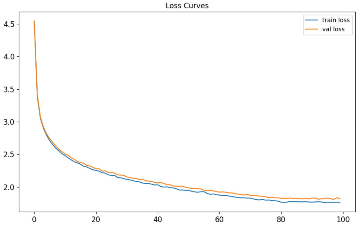
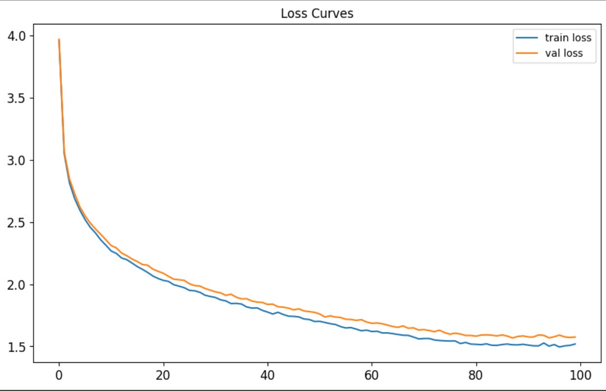
Running this for 100k training steps bring the final validation loss down from 6.4 to 4.4. Here are the loss curves:
It also lowered the perplexity from 424 to 22. Now let’s check a sampled story:
Story time: „h3I\vŠâªâ¤š°FA7G
'½ndS4 m tt .elhIeidoioms e oaiydsseJgd
tceo,ty,
wSns itt h hs ud rli eh rndg ee l S ,yed dp i ra cam d"ae.Sodtro,eo ehoh h ahd lstbr tuv t,yeo t ho"
hlbLsth usrnwymdecr oi erswiii Tdw.we onhaourdh wtko temn epea shoaws ecstSapniade rg a ,ehaf e scn ehdg dat me i'hg osutah yaaaetsds
het atw obn h usuyhwuknnlnus hla isttctioih oer T r olwa hi uuryTt m twannaw ee.ahem, rsf nta snioe as iep hirigyn!e o ut tSeos dcstagbui"bSn"tyawlud
h ueyi rtocg ar emtaae aoni rl"ag l fhn Tt b pte mbmah ahwt"aueEiva ai rv" hswr!eA .ekga ote edu, hyw ohoee?T wtt lrthnecmb'au hlend tytiuwdld E a,snaus.tc lddd otnHsbgre"tasdhidrMdtr ebtrhasa esc aa
meT mntyldmmpu s"
esnty.csyeâa itielt nh a tp ol oesn iie obgfeS.sogskB cen
hdiaes e hssuo.
As we can see, our dream of Skynet is still in the far distant future, however we are making progress; the model is starting to learn what appears to be the ASCII character range, word boundaries, and punctuation. Since our validation loss is still close to the training loss, we have room to simply add more parameters before overfitting takes over. We could do this by adding additional layers or increasing the embedding and/or hidden dimensions.
But before we throw even more capacity at the problem, I want to dig into the flow of various data streams throughout the network. The behaviors of these streams of data, both in the forward and backward direction, are called the training dynamics. In order to train deep networks, we have to ensure that the training dynamics are stable, otherwise gradient descent will diverge. If gradient descent diverges, then our model fails to learn anything useful. The most common culprit of unstable training dynamics are unstable gradients.
The Gradient Must Flow
Like the spice of Arrakis, the gradients within our network have to flow to each of the parameters in order for them to learn. Recall the update formula:
If p.grad is zero, the parameter value (p.data) doesn’t change. Likewise, if p.grad is too large, it can teleport us to completely different parts of the loss landscape without ever settling down into a minimum. So we need to understand and monitor the gradient values for each layer to ensure they don’t become degenerate.
For our model, we are using linear layers followed by tanh activation. To understand the gradients through these layers, we can analyze the graphs of tanh and its derivative:
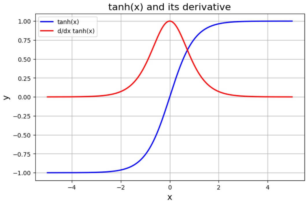
We can see the derivative (in red) vanishes to 0 as the absolute value of the input increases beyond roughly 3. This region beyond |3| is the saturating region of the tanh activation. What is the input to our tanh? The input is the output of the linear layer y (also called the preactivation):
So as soon as the absolute value of y gets larger than 3, tanh itself becomes saturated, and the gradient on the tanh for that value will be essentially 0. This problem compounds in backpropagation with each additional layer because of the chain rule, which is multiplicative:
When the gradient of tanh is 0, the middle term dz/dy is 0, causing the entire expression to be 0. This 0 gets propagated down to the child nodes in the computational graph (i.e. layers which are closer to the beginning), causing learning to stagnate in these deeper layers as well.
Visualizing Gradients
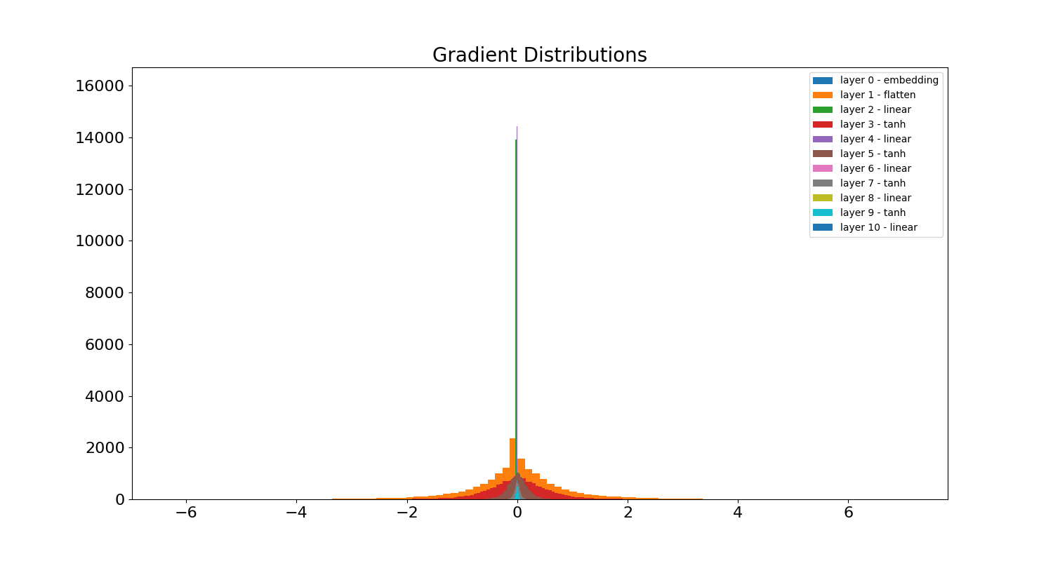
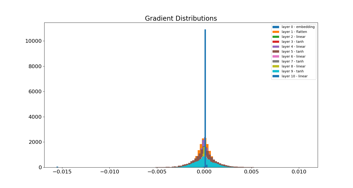
To gain more intuition for this problem, it helps to visualize the gradient values of different layers at various steps during training. Below is a histogram of each layer’s gradient after training for 100k steps. You can see from the spikes in the middle that several layers’ gradients have vanished substantially:
We can double-click on these layers to see the evolution of the gradient for each neuron at various training steps. Below is the evolution of the gradient of the first linear layer. As the gradient tends to 0, the color of the corresponding point in the heatmap tends to purple. A vertical column of purple indicates a completely dead neuron - no gradient is flowing through it. The x-axis indicates the neuron and the y-axis is the batch:
Below is the evolution of the last linear layer, i.e. the output layer. You can see it fares a little better than the first linear layer, yet still only has a few surviving neurons:
So what can we do to ensure better gradient flow? There are many options, more than I can cover in this post. However they mostly revolve around the same fundamental idea: we need to avoid inputs which lead to saturated non-linearities. In our example, this means avoiding too many inputs whose absolute value is greater than roughly 3, beyond which the derivative of the non-linearity, tanh, is zero. Other non-linearities will have different bounds, but the need to avoid these bounds is the same. Below we will look at a few techniques that are useful for mitigating excessive saturation.
Xavier Initialization
Glorot and Bengio figured out that for tanh activations1, keeping the variance of the preactivations close to one for every layer helps to create more stable gradient flow. The reason is that assuming the preactivations have mean 0 and variance 1, then approximately 95% of all values lie within the interval [-2, 2], thus 95% of the values will stay within the non-saturated region of tanh.
If we assume the inputs and weights are independent with mean 0, then we can calculate the variance of the jth neuron (assuming zero bias for simplicity):
If we further assume the weights and the inputs have a constant variance Var(W) and Var(x), respectively, then we can derive an expression for Var(W) which provides a variance of 1 on yj:
So for initialization we can choose a W such that the variance of W depends on the fan-in (n) of the layer, as well as the variance of the input. The input could be the actual input, or it could be the activation from a previous layer. This underscores the importance of normalizing the data input to the network - doing so ensures the assumptions of the above calculations are met and that the chain of variances can be one throughout the network. This is essentially what so-called “Xavier initialization” does.
After re-training the model with PyTorch’s xavier_uniform_ on each linear layer, we get the following loss curve:
Notice the initial loss is much closer now to the expected baseline of ln(nr_classes) = ln(174) = 5.15. This change also brought the final validation loss down from 4.4 to 1.9 and the perplexity down from 22 to 5.73. Let’s sample a story:
Story time: 1ap ue was laghoned thain hit wayl Ieind om tearouly ss og otciout the ton ittligher and reined veru†ne low at wis pois, shay dove. Eher weorej Io hatd ast Iraw. RWy and her hebfat hemstily hecrpeneser with he was and and hewtur to nacked itho
" brat. He ane sard a dore aflyen sconed. That was in tad, thery are sus is the boun hit'ur wor't beap ala bimtterigit on the bolea ci'rus. Tthe twand.
We. hem, tharent Ting to pave puririgen.
Aut theor dact gerilbeghty was ho sey herocghtryemeree to hackri" gily fin the dparpmbmas and "aver Iaw iore" haw so loqk ver"eded they dobee tike therthe cablaw hernd tearpund a hays. Th. The ded to shire raschilred boZ theas to chaaned Timmyy whipg saine. They yin tigingt nog her oldong to he cogie took the cent oudines a histo.
Woge hiund have hake, "athee lilly can sever bucher. Th they jaly Sveol.
Still nonsense! But also much better. We see some actual English words now and both sentence and paragraph structure starting to emerge. All that just from specially chosen initialization values. Now let’s check the gradients. Here is the overall distribution:
We can see the peak is lower (from around 15000 to roughly 12000), and there appears to be just one layer, the embedding layer, which has significantly vanished gradients. This perhaps isn’t surprising, because it is the last layer in gradient descent, so any near-zero multiplicative affects from its ancestors in the computational graph are magnified there. Here is the evolution of the gradients for layer 2, the first linear layer:
Interestingly, the gradients start out closer to zero in the first step relative to the non-Xavier init model. However as training continues, the gradients’ magnitudes appear to get slightly larger on average, increasing at each step. If you look at the last frame, it looks like no neurons are completely dead - there are at least a few batches providing non-zero gradients.
There is alot more to initialization than was covered here. Xavier init is good for activations that are symmetric around 0, whereas Kaiming init is better suited towards asymmetric activations like the ReLU and its relatives.
One shortcoming of these special initialization techniques is they obviously only occur once. This can cause the network, especially deep networks, to have drifting activations over time. This drift can venture into saturating or exploding regions of activations, causing unstable gradients. One mitigation to this is to add normalization dynamically at each layer so that the inputs to the subsequent non-linearity stay in the activated region.
Layer Normalization
Many different types of normalization techniques exist. And you can apply normalization to different types of data - weights, preactivations, gradients, input data, etc. Layer normalization typically applies to the preactivations, i.e., the output y of the linear layer:
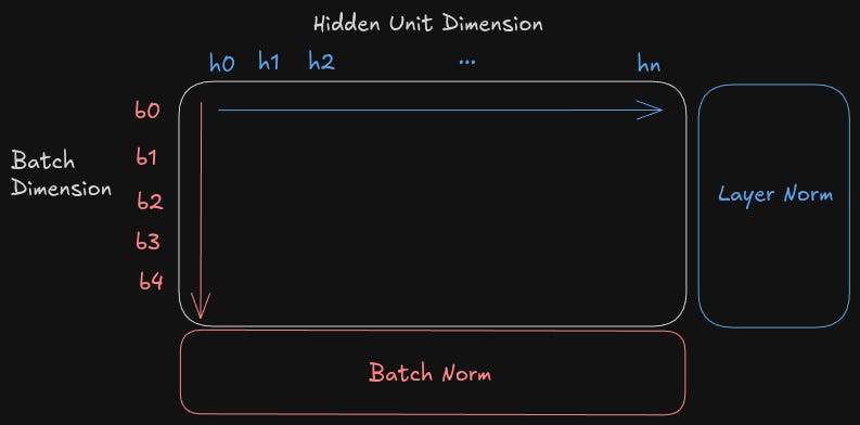
Layer Normalization applies this normalization across the hidden unit dimension. This means the average and variance are computed across each neuron in a single batch. This is opposed to Batch Normalization, which normalizes across the batch dimension:
The advantage of layer norm over batch norm is that batch norm requires keeping a running average and variance throughout training so that it can be used later during inference. The reason is that inference has to gracefully handle a batch size of 1, but the average and variance over one element is at best noisy and at worst meaningless. So we have to retain the statistically significant batch statistics computed during training and reuse them during inference. On the other hand, layer norm works with any batch size, including batch size of 1 during inference and doesn’t require any special state between training and inference. The implementation is straightforward:
| class LayerNorm(): | |
| def __init__(self, device, num_features): | |
| self.out = None | |
| self.gamma = torch.ones(num_features, device=device) | |
| self.bias = torch.zeros(num_features, device=device) | |
| def __call__(self, x: torch.Tensor): | |
| assert x.ndim == 2 | |
| H = x.shape[1] | |
| avg = x.mean(dim=1, keepdim=True) | |
| std = torch.sqrt(1 / H * ((x - avg)**2).sum(dim=1, keepdim=True)) | |
| self.out = (x - avg) / std * self.gamma + self.bias | |
| return self.out | |
| def params(self): | |
| return [self.gamma, self.bias] |
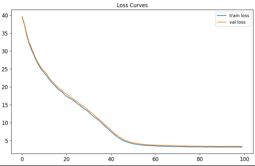
Let’s see what happens when we add LayerNorm after each linear layer and retrain. The loss curves are reaching a slightly lower minimum (and also slightly overfitting):
The final validation loss improved from 1.9 to 1.7. Perplexity improved from 5.73 to 4.50. Ok, now grab some coffee! It’s time for another story:
Story time: Once dook had rine. It was tore on. They fubbe= ef, storisk âun wookgar. The fabiing. He soulld eed sou jrean frea toy tayt their to so she prcedadn- and suym haw seare a vene ily. Polly wari. They were mad a wert to xime, the veasen" and grien to but furnyt want to sed talked a may.
The grid a foll. The "iling. %o loon a with ray fft. Tre sly call. He dayz away hoff the perter. The whone her to saibry. The smuny. She by timpy something to seve
fee the ground a cime then gratest ands and a with his wood! One day plays garond to curprasy was so ine of the back to take a smiled. Ore lefyor her!" Soras ecried. Jon the will and adpoly toor lantend his and story."
Hey look at that, dook had rine! We’re getting more words now. And the early hints of a coherent story are taking shape. A lot of the words are nonsense still, but the sentences appear to have a structure with basic subject-verb agreement.
Here are the gradients at the end of training:
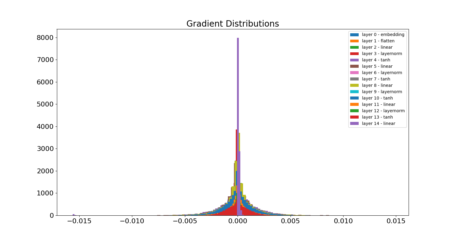
The peak is lower, down to 8000 from around 12000. It looks like many of the layers have a decent spread around 0 as well. Here is the evolution of the gradient of layer 2:
Once again we see the gradients slightly increasing in a controlled way, and no neurons appear dead on any of the steps.
Conclusion
In this post we’ve focused on understanding gradient flow and deployed two techniques for stabilizing gradients during training: Xavier initialization and LayerNorm. Of course there are other aspects of the training dynamics we could look at, especially the parameter update size and learning rate. There are also architectural tricks like residual connections. These connections provide an additional path for gradients to flow back to deep layers. They work by providing a direct linear path from one deep layer to another closer to the output, thereby bypassing the sequence of non-linearities and repeated matrix multiplications that can lead to instabilities. We applied these techniques to language modeling, but they apply generally to all neural networks. In the next post we will further improve the performance of our model by leveraging recurrence.
Their findings applied to activation functions that are symmetric around zero, not just tanh