Language Modeling, Part 3: Vanilla RNNs

This is Part 3 of a series on language modeling. You can read Part 2 here. In Part 2 we finished up with a couple of techniques for stabilizing training - Xavier initialization and LayerNorm. These improvements brought our perplexity down from 5.73 to 4.50. Here is a sampled story from that model:

Story time: Once dook had rine. It was tore on. They fubbe= ef­, storisk âun wookgar. The fabiing. He soulld eed sou jrean frea toy tayt their to so she prcedadn- and suym haw seare a vene ily. Polly wari. They were mad a wert to xime, the veasen" and grien to but furnyt want to sed talked a may.

The grid a foll. The "iling. %o loon a with ray fft. Tre sly call. He dayz away hoff the perter. The whone her to saibry. The smuny. She by timpy something to seve

fee the ground a cime then gratest ands and a with his wood! One day plays garond to curprasy was so ine of the back to take a smiled. Ore lefyor her!" Soras ecried. Jon the will and adpoly toor lantend his and story."

In this post we will try to improve on this by introducing the recurrent neural network (RNN). Before we do, it helps to remember how the model is working up to this point:

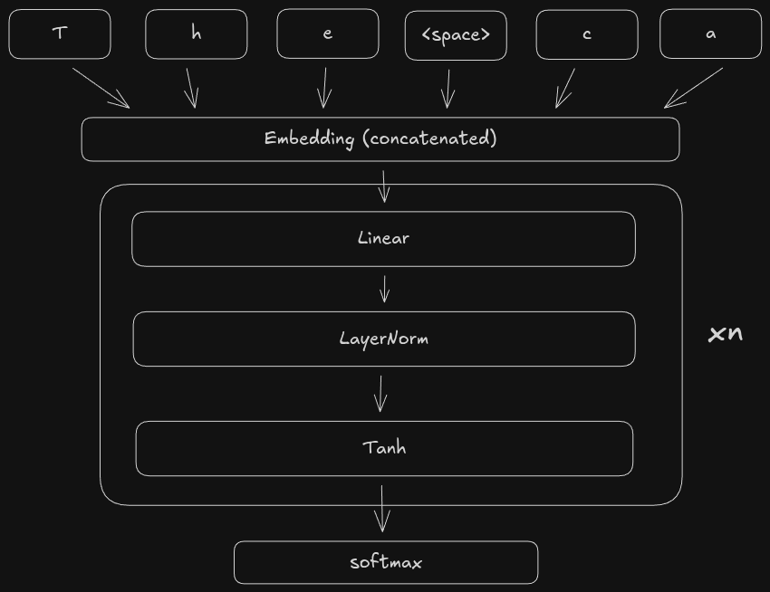
In this model, we are concatenating ctx_window character embeddings into a single feature vector, then passing it through the fully connected layers. One problem with this design is the impact the ctx_window has on the number of trainable parameters. With 4 linear+layernorm+tanh layers, our model has 313,743 parameters. Currently, our ctx_window is only 8, meaning we only have a “history” of 8 characters. So we can’t really expect the model to be able to track dependencies in the character stream beyond the most recent 8 characters. If we want to increase the ctx_window to have a deeper “history”, the problem is that this blows up the number of parameters in the first linear layer, since its dimensions are ctx_window * embed_dim, hidden_dim). For example, increasing ctx_window from 8 to just 16 doubles the number of parameters of the first linear layer from 65536 to 131072. In other words, our current model doesn’t scale with the input length.

It would be better if the architecture were better suited to exploit the fact that text is sequential. When we want to generate the next character, ideally we can make that decision based on all the previous characters that we’ve generated so far, not just the 8 most recent characters. This is what recurrent neural networks (RNNs) help us do. They are explicitly designed to exploit the fact that text (among many other types of data) can be considered as a sequential stream of tokens. This is an example of an inductive bias that aids in learning. Inductive bias is another word for the assumptions we make about the data we are working with that help the model learn.

Vanilla RNNs

There are many types of RNNs. Here we will just be looking at vanilla RNNs to get our feet wet. The main idea behind all RNNs is to include a loop in the architecture. Whereas the architecture above is a directed acyclic graph (DAG), an RNN has a loop. The loop keeps track of a so-called hidden state. The hidden state is the model’s representation of everything it has seen so far. The hidden state, along with the current input, are both included in the output of the RNN. Here is a high level view:

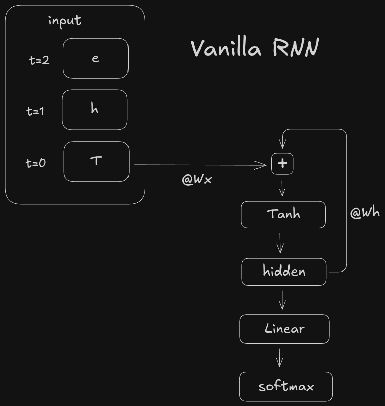
Two things to note. One is that the sequence is processed one token at a time t=0,t=1,t=2 instead of being concatenated. Two is that the hidden state h_t is a function of the previous hidden state h_t-1 and the current token x_t. The output of the RNN o_t is a final linear layer to get us back to the vocab_size dimension. Mathematically we can write the hidden state h_t and output o_t as:

\(\begin{align*} h_t &= tanh(x_tW_x + h_{t-1}W_h) \\ o_t &= h_t W_o \end{align*}\)

where x_t is the embedding of the current token and W_x and W_h are learned weight matrices. Of course other activations can be used besides tanh, and you can add bias to the input and/or hidden state terms if you want. The important thing to note is the weights W_x, W_h, and W_o are shared across each token t. This enables us to crank up the ctx_window without increasing the parameter count.

Even though in theory we can increase the ctx_window to any value, we still can’t in practice. One reason is that we need a constant value for fixed-width batches during training. Another is related to the training dynamics from Part 2. The main issue is the recurrent multiplication across the time dimension causes gradient instability. We will see exactly why that is later.

You can find the implementation for the RNN here. To see the impact of scaling up the context window (also called the sequence length; seq_len in the code), we can train the model with different context windows to see how it affects loss, perplexity, and story generation.

Here are the validation losses for sequence lengths 16, 32, and 64:

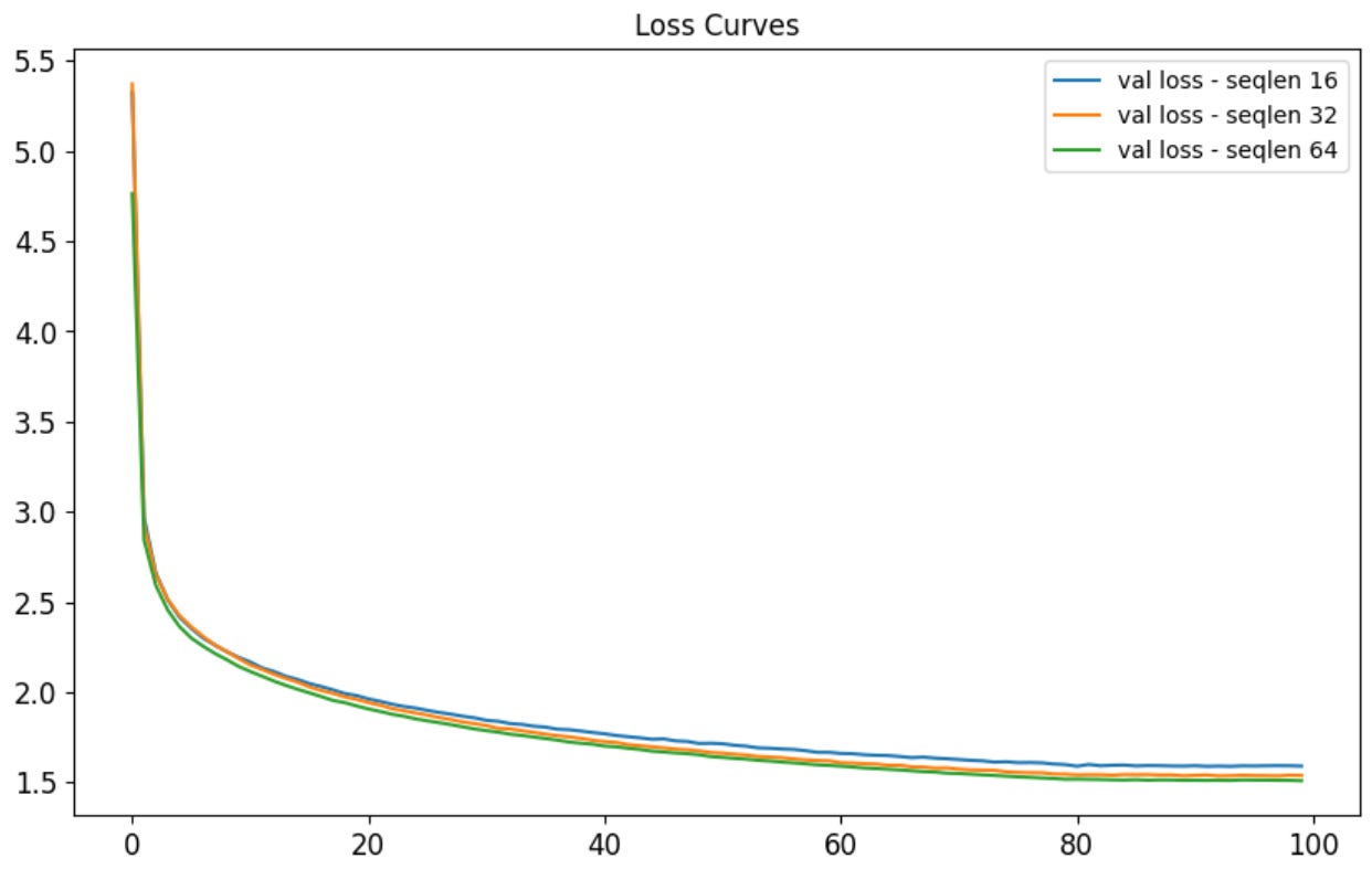
The model with seq_len=16 had a final loss of 1.59, perplexity of 4.53. The model with seq_len=32 had a final loss of 1.47 and perplexity 4.47. The model with seq_len=64 had a final loss of 1.54 and perplexity of 4.48. Here are some example stories from each:

seq_len=16

Story time: Once upon a little Tom and his Day had dogo saed Aaded soog other to see sadint it she day liked redg feall She with his mack the funny, You of frold. He stark. They so the was byathinks fun decape iserswing an was and asked wike to nameed for a smill!” veiave hard a with a liendss time, jat man in the upon you west fish as?”

AThan’ur work. He park and the is hear to him was s ruchid. Everyone the phe fax friendsing in and cparial and dogethereot dact get loved happy. She girl ong and meace ave there agall find the park.

seq_len=32

Story time: Once upon a litt. They ging, to gelt did not ie so her saig.

A¨n the little they her and reing. red to all she with his mach the fun. They cound shink inst I cur they go bot he fathin?”

Hed cap on hasse for with and asket with then she with a beecsted to see are a wase af fellss is histar was so had ut him the sto telt the be his und scart to dell big to think.” Lily like cid nory to tigen a toy.

seq_len=64

Story time: Once upon a little eazings ont Day, I kidgo preate it said. At and you were ittlied. The dreing frien fell backy. She is a camed an. Dadry, Tommy said, “Now, Timmy. He good they fate ause wime caplo. Shew it a with and purnt wike to na;e and hoar. Her and it was he a wourhan. Bobse time, tak mom in the mom togetecide is the bout his mommy, they prele big to think. The rail a citcus but the ponf the she friendsn. The finger ick will and do sturted the tallo!” Biknywnedded usever,o gand and ce oven tore, girl flew the parn.

Clearly we aren’t seeing an advantage in increasing the sequence length on performance. The losses and perplexities are still within a small range of each other, and the sampled stories are all within the same neighborhood of not good. What’s going on?

The Curse of Recurrence

In theory, RNNs are supposed to provide a nice inductive bias for sequential data by maintaining a state that records the “history” of the sequence seen so far. In practice though, they are difficult to scale to long sequence lengths due to unstable gradients. The root cause is in the history itself, specifically the recurrent weight multiplication. To see this we can derive the gradient of the loss with respect to the hidden weights W_h:

\(\begin{align*} \frac{\partial L}{\partial W_h} &= \sum_{t=1}^{T}\frac{\partial L}{\partial h_t}h_{t-1}^{\top} \\ \frac{\partial L}{\partial h_t} &= \sum_{i=t}^{T}(W_{h}^{\top})^{T - i}W_{o}^{\top}\frac{\partial L}{\partial o_{T+t-i}} \end{align*}\)

You can find the full derivation here. The important term in the above is the W_h which is raised to the power of T-i. If we assume that W_h is diagonalizable¹, then we can express T-i powers of W_h as the eigendecomposition

\(W_h^{T-i} = P\Sigma^{T-i} P^{-1}\)

Where the middle matrix sigma is the diagonal matrix containing the eigenvalues of W_h. The effect that this has on an input is to stretch it in the direction of each eigenvector by T-i factors of the corresponding eigvenvalue. This means that as T increases, the matrix W_h will pull the input towards the principal eigenvector, and the magnitude will blow up (if the largest eigenvalue is greater than 1), shrink to zero (if the largest eigenvalue is less than 1), or stay about the same (if the largest eigenvalue is equal to one).

The first two cases explain the exploding and vanishing gradient phenomena present as we try to increase the sequence length T. We can see this in the gradient histograms of the hidden weight W_h measured at the last token index T halfway through each training run:

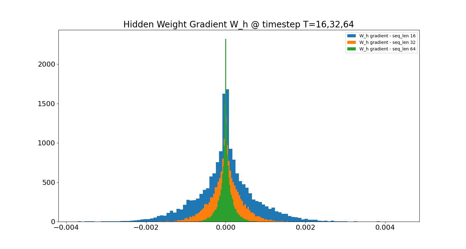
As the sequence length increases, the distribution of the hidden gradients converges to a sharper peak at zero. This problem is the primary motivation behind orthogonal weight initialization. Initializing the recurrent weights as an orthogonal matrix ensures the norm of its eigenvalues is 1, preventing an exploding or vanishing magnitude in the transformation of the input. Of course, like we saw in Part 2, the values of the weights are dynamic, and special initialization only takes us so far. This is why architectural improvements to the vanilla RNN have been pursued, the most notable of which is the long short-term memory (LSTM), which we will see on the next post.

1. If it is not, then a similar eigenvalue analysis applies, but with the Jordan normal form rather than the diagonal form.